Calibrate Scores, Not Sensitivity: Anomaly Detection Tuning for SREs

The most reliable path to fewer false alarms is to calibrate model scores into a stable percentile space, layer on adaptive thresholds using extreme value theory or dynamic percentiles, and add a second-stage confirmation filter before anything reaches a human. Before touching a single hyperparameter, measure your current false-positive rate, your AUC-ROC and PR-AUC baseline, and your true anomaly prevalence. Those three numbers tell you whether you have a detector problem or a threshold problem.

TL;DR:

Calibrating scores into percentile space and adding adaptive thresholds reduces false positives, but the choice of method depends on anomaly rarity and data distribution.

Starting with statistical, tree-based, or density methods depends on data shape, latency needs, and complexity, with simple models often outperforming heavy ones in low-latency scenarios.

Building a repeatable workflow involves establishing a baseline, splitting data by episodes, limiting hyperparameters, calibrating scores, and validating through replay to ensure stable improvements.

Thresholds based on extreme value theory or percentiles require regular recalibration, especially when true anomaly prevalence shifts, to avoid excessive false alarms or missed incidents.

Incorporating operator feedback, multi-channel corroboration, suppression rules, and domain knowledge effectively reduces false positives without sacrificing detection recall.

What Is Anomaly Detection Tuning?
Which Anomaly Detection Techniques Should You Start With?
How Do You Build a Repeatable Tuning Workflow?
How Do You Choose the Right Detection Threshold?
How Do You Cut False Positives Without Losing Recall?
Which Metrics Actually Prove Your Tuning Worked?
How Do You Keep a Tuned Detector Accurate Over Time?
How Netverge Applies These Tuning Patterns in Production
What Preprocessing Actually Improves Anomaly Detection?
How Should You Handle Imbalanced Data While Tuning?
Why Does Prevalence Change Your Tuning Decisions?
How Do You Bring Domain Knowledge Into Tuning?
How Do You Tune Anomaly Detection at Scale?
What Should You Prioritize in Your First 90 Days?
How Netverge Fits Into a Production Tuning Workflow
Sources
FAQ

What Is Anomaly Detection Tuning?

Anomaly detection tuning is the process of adjusting a detector's parameters, thresholds, and post-processing logic so it flags real problems without drowning operators in noise. It covers everything from picking the right base algorithm to calibrating raw scores, setting sensitivity, and layering suppression rules on top of the model's output.

Most teams treat tuning as a single knob: turn sensitivity up, get more alerts; turn it down, get fewer. That framing is why so many production systems either miss incidents or bury their SOC teams in noise. Real anomaly detection optimization touches the whole pipeline: how you preprocess data, which detector family you choose, how you calibrate its scores, where you set the threshold, and what happens between a raw flag and a human seeing it. Get the architecture right and sensitivity becomes a much smaller decision.

Which Anomaly Detection Techniques Should You Start With?

Your data's shape and your latency budget should decide your starting detector, not habit or whatever library your team already has installed. Each method family carries a distinct set of knobs, and knowing which ones actually move the needle saves weeks of blind grid searching.

Statistical methods (z-score, STL decomposition): fast, interpretable, and a reasonable first pass on seasonal metrics. The key knobs are the rolling window length and the seasonal period; get the period wrong and every threshold downstream is meaningless.
Tree ensembles (Isolation Forest): strong general-purpose choice for tabular or multivariate data without strong temporal structure. Tune the contamination parameter, number of trees, and subsample size; contamination is the one most people set wrong because it is treated as a known constant rather than an estimate.
Density methods (LOF, ECOD): effective when anomalies cluster in low-density regions of feature space rather than appearing as simple outliers. Neighbor count (for LOF) and feature scaling matter more here than almost anywhere else in the pipeline.
Reconstruction methods (autoencoders): useful on high-dimensional or image-like telemetry where you expect nonlinear structure. The reconstruction error threshold and the latent dimension size are the two levers worth your time.
Forecaster plus residual analysis: a strong default for time series with real seasonality, since you tune the forecaster's accuracy separately from the anomaly threshold on its residuals.
Transformer-based multivariate models: worth the complexity only when you have many correlated channels and enough history to train on; shingle or window size dominates performance more than architecture depth.

If you are running low-latency streaming telemetry, forecaster-plus-residual or lightweight statistical methods usually beat heavier reconstruction models on cost and interpretability, even when the heavier model scores slightly better offline.

How Do You Build a Repeatable Tuning Workflow?

A repeatable workflow separates real improvement from a threshold that happens to look good on last week's data. Skipping this step is the single most common reason teams re-tune the same detector every quarter without ever getting more confident in it.

Establish a baseline. Record AUC-ROC, PR-AUC, prevalence, and a flag-everything F1 score before changing anything. A "flag-everything" baseline sounds silly, but it exposes exactly how much credit your detector deserves for beating a trivial system.
Split by episode, not by random window. Randomly shuffled train/test splits leak information across an anomaly episode and inflate every metric that follows. Group each incident into a single episode and split on episodes.
Run window sensitivity experiments. Test two or three window or shingle sizes against two or three detector families before committing. This tells you whether a poor score is a model problem or a windowing problem.
Limit hyperparameter search to 3 to 5 knobs. Random or Bayesian search across a handful of high-impact parameters outperforms exhaustive grids that waste compute on parameters with little effect, a pattern AWS's SageMaker guidance echoes for log anomaly pipelines.
Calibrate scores, not labels. Convert raw model output into percentile ranks and store the raw scores for future recalibration. Never bake a hard label into the model itself; keep the decision function separate so thresholds can move without retraining.
Validate through replay. Run the tuned pipeline against historical traffic with known incidents injected or replayed, rather than trusting a single static test set.

Pro Tip: Before adjusting any hyperparameter, check whether your training window aligns with the system's real seasonality. A practitioner review of window alignment found that fixing seasonality mismatches often produces bigger stability gains than an entire round of hyperparameter search.

How Do You Choose the Right Detection Threshold?

Threshold selection determines whether your calibrated scores translate into a usable alert stream, and small threshold changes can swing your false-positive rate dramatically, according to research on anomaly scoring methods. Three approaches cover almost every production scenario.

Extreme value theory (EVT): models the tail of the score distribution directly, which suits systems where true anomalies are rare and you need a threshold grounded in tail probability rather than an arbitrary cutoff. Set a target risk ratio, such as one false alarm per thousand observations, and let EVT derive the corresponding score cutoff.
Percentile-based thresholds: the practical default when you have no labels at all. Flagging anything above the 99.5th percentile of a rolling score window is crude but auditable, and it adapts naturally as you update the rolling window.
Recall-at-fixed-precision sweeps: when you do have labels, sweep the threshold and report recall at a fixed precision (say, 90%) rather than chasing a single F1 number that hides the tradeoff.
Temporal smoothing via EWMA: smoothing residuals with an exponentially weighted moving average before thresholding removes single-point spikes that would otherwise trigger alerts. The smoothing window "h" needs its own small sweep. Too short and you smooth nothing; too long and real incidents get averaged away.

Small threshold shift, big consequence: analytic reviews of anomaly scoring consistently find that marginal threshold adjustments produce outsized swings in false-positive rate, which is why threshold and scoring decisions deserve as much attention as the detector model itself.

How Do You Cut False Positives Without Losing Recall?

Structural mitigation, not sensitivity reduction, is how mature teams get their false-positive rate down without missing real incidents. Turning down sensitivity is the crude version of this problem; architecture is the disciplined version.

Two-stage confirmation. Train a secondary classifier on the true positives and false positives your primary detector already produced. This FADFPM-style approach, validated for predictive maintenance, can meaningfully cut false alarms because the second stage learns the specific error pattern of your first detector rather than a generic rule.
Multi-modal or fleet-level fusion. Require corroboration across independent channels, such as vibration, latency, and temperature, before raising an alert, since combining independent sensing modalities prevents a single noisy sensor from triggering a false alarm on its own.
Suppression logic. Deduplication, cooldown windows, and hysteresis (different thresholds for entering versus exiting an alert state) stop the same underlying issue from generating a dozen tickets.
Alert aggregation. Roll related flags from correlated channels into a single incident rather than paging on every individual signal.
Human-in-the-loop feedback. Capture operator dispositions (confirmed, dismissed, duplicate) as labels and feed them into weekly retraining. Track false-positive rate and triage time as your two core KPIs.

Pro Tip: Treat operator dismissals as gold-standard negative labels. Most teams throw this feedback away, then wonder why their second-stage classifier has nothing better to learn from than the original detector's own blind spots.

Adaptive thresholds paired with fleet comparisons and human feedback loops remain among the best-validated approaches to reducing false alarms in industrial anomaly detection, and the pattern holds well beyond manufacturing.

Which Metrics Actually Prove Your Tuning Worked?

AUC-ROC and PR-AUC are your primary metrics because both are threshold-independent, which means they measure the detector's ranking ability separately from whatever cutoff you eventually choose. An IETF draft on network anomaly evaluation treats AUC-ROC as the metric of record specifically because it survives changes to your threshold decision.

Operational metrics matter just as much once a threshold is set:

Recall-at-fixed-precision: how many true anomalies you catch while holding false-positive rate to a level operators can tolerate.
PR@k: precision among your top-k highest-scored alerts, useful when triage capacity is limited.
Episode-level detection rate: whether you caught the incident at all, not just individual anomalous points within it.
Detection latency distribution: how long, on average and at the tail, before a real incident gets flagged.

Watch for point-adjustment inflation. Some evaluation pipelines count a single correct flag anywhere inside a known anomaly window as a full detection, which lets weak detectors look far stronger than they are. Operator-interest-based metrics were built specifically to correct for this. Always report prevalence alongside F1, since a rare-event dataset produces a misleadingly low F1 floor even for a good detector.

Benchmarking element	Why it matters
Episode-based splits	Prevents leakage across a single incident's data points
Fault injection or replay	Tests against known ground truth instead of assumed labels
Multiple window sizes	Confirms results aren't an artifact of one arbitrary window choice
Run-to-run dispersion	Exposes threshold fragility that a single point estimate hides

How Do You Keep a Tuned Detector Accurate Over Time?

Drift detection and a defined retraining cadence are what keep yesterday's tuning from becoming tomorrow's noise generator. A detector tuned in January against January's traffic patterns will quietly degrade as your infrastructure, traffic mix, or seasonality shifts.

Run a population stability index or Kolmogorov-Smirnov test on key feature distributions daily for high-velocity systems, weekly for stable ones.
Retrain weekly for systems with fast-moving traffic or topology changes; monthly or quarterly is usually sufficient for stable, low-drift environments.
Consider online learning algorithms only when drift is continuous rather than occasional. Full retraining is simpler and easier to audit for everything else.
Set an alert budget per team per week and hold triage to a defined SLA. An unbounded alert queue defeats every tuning effort upstream of it.
Version every model, threshold, and calibration change so you can replay against historical traffic before a rollout goes live. This is how configuration drift tracking earns its keep operationally, not just conceptually.

How Netverge Applies These Tuning Patterns in Production

Netverge's architecture mirrors the recommended pattern above rather than treating tuning as an afterthought. Vergepoints provide the multi-sensor corroboration this guide recommends, feeding independent signal channels into a shared calibration layer instead of relying on a single noisy metric.

Some systems run second-stage confirmation on flagged events before they reach a ticket queue.
Suppression and deduplication logic can apply automatically across correlated alerts from the same root cause.
Operator dispositions may feed back into ongoing calibration rather than sitting unused in a ticket log.

Teams that add a confirmation layer on top of a single detector typically see a meaningful drop in false-positive rate alongside improved recall at a fixed precision target, consistent with the two-stage patterns described in FADFPM research.

What Preprocessing Actually Improves Anomaly Detection?

Feature engineering decides how much signal your detector can even see, before any tuning happens downstream. Raw telemetry rarely arrives in a shape a detector can use well.

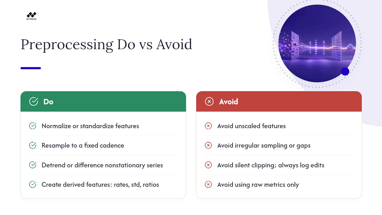
Normalize or standardize features so that a metric measured in the thousands (bandwidth in bits) doesn't drown out one measured in single digits (a latency z-score), since distance-based methods like LOF are especially sensitive to scale mismatches. Resample irregular time series to a fixed cadence before windowing; gaps and jitter in sampling intervals corrupt shingle-based features in ways that look like anomalies but are really data artifacts. Difference or detrend series with strong seasonal or trend components before feeding them to a detector that assumes stationarity, or use a forecaster-plus-residual approach that handles this implicitly.

Engineer domain-specific derived features rather than relying only on raw metrics. A rate of change, a rolling standard deviation, or a ratio between two correlated channels often carries more anomaly signal than either raw input alone. For multivariate systems, correlation-based features (how far a metric has drifted from its usual relationship with a peer metric) frequently catch anomalies that univariate thresholds miss entirely. Cap or clip extreme outliers during training data preparation, but log what you clipped. Clipping the wrong thing silently removes the exact signal you are trying to detect.

What Preprocessing Actually Improves Anomaly Detection? — overview diagram

How Should You Handle Imbalanced Data While Tuning?

Anomaly detection is inherently an imbalanced-classes problem, often by several orders of magnitude, and pretending otherwise is what wrecks most naive tuning attempts. Standard classification tuning advice ("balance your classes with oversampling") often does not translate cleanly here because the rare class is defined by being rare and unusual, not just underrepresented.

Avoid naive oversampling of anomalies (SMOTE and similar techniques) unless you have validated it does not create synthetic anomalies that look nothing like real ones. For genuinely unsupervised detectors, imbalance is handled implicitly through the contamination parameter or percentile threshold rather than through resampling. For semi-supervised or two-stage classifiers trained on labeled true and false positives, weight your loss function or use precision-recall-aware metrics rather than accuracy, which is meaningless at extreme imbalance ratios. Stratify your episode-based splits so that both training and validation folds contain a representative number of anomaly episodes, not just a representative number of anomalous data points. Track class ratio explicitly as a reported metric alongside every tuning experiment, since a threshold that looks stable at one prevalence level can behave very differently if the underlying rate of anomalies shifts.

Why Does Prevalence Change Your Tuning Decisions?

The rarer your true anomalies, the more your metrics and thresholds need care, because low prevalence mechanically punishes even a well-tuned detector's F1 score. This is not a flaw in the detector. It is a property of the math.

At 0.1% prevalence, a detector with strong ranking ability (a healthy AUC-ROC) can still post a mediocre F1 score simply because false positives, even at a low rate, vastly outnumber the rare true positives in absolute terms. This is exactly why threshold-independent metrics like AUC-ROC and PR-AUC matter more than F1 for imbalanced anomaly problems, a point the IETF evaluation methodology makes explicit by requiring prevalence disclosure alongside any reported score.

Prevalence should also inform your threshold choice directly. A percentile-based threshold set at the 99th percentile implicitly assumes roughly 1% of your data is anomalous. If your real prevalence is closer to 0.01%, that threshold will flood you with false positives regardless of how good the underlying detector is. Recompute your target percentile whenever you have reason to believe true prevalence has shifted, and treat prevalence as a monitored metric in its own right, not a one-time assumption baked into a config file at launch.

How Do You Bring Domain Knowledge Into Tuning?

Domain constraints should override statistically "optimal" parameters whenever the two conflict, because a threshold that scores well offline but ignores known operational reality will fail the moment it meets real traffic. This is where anomaly detection optimization stops being a purely mathematical exercise.

If your team already knows that a maintenance window every Sunday night produces legitimate traffic dips, encode that as a suppression rule or a seasonal feature rather than hoping the model learns it from six months of data. If certain metrics are known to be noisy at specific times of day (a batch job, a backup window), incorporate that as a time-aware threshold rather than a flat one. Subject matter experts often know which combinations of signals matter together (a latency spike alone means nothing, but a latency spike plus a packet loss increase means something) and that correlation knowledge should shape your feature engineering before it ever reaches the model. Build a short feedback loop where operators can flag "this alert type is structurally wrong" separately from "this specific alert was a false positive," since the first signals a tuning problem and the second is just normal noise. Domain knowledge is cheapest to apply early, in preprocessing and feature design, and most expensive to retrofit later as a patchwork of suppression rules.

How Do You Tune Anomaly Detection at Scale?

Streaming and large-dataset scenarios change which tuning techniques are even feasible, since a technique that works beautifully on a batch dataset can be computationally impossible at real-time scale. This is where many otherwise-correct tuning plans fall apart in production.

Favor incremental or online-capable algorithms (streaming z-score, online Isolation Forest variants) when data volume prevents full retraining on a regular cadence, but validate that their approximations do not silently degrade your AUC-ROC compared to a batch equivalent. Downsample or aggregate at the ingestion layer rather than the detection layer when raw volume is the bottleneck. Detecting anomalies on one-minute rollups instead of raw per-second data often loses little real signal while cutting compute dramatically. Partition detection by logical grouping (per device, per site, per tenant) rather than running one global model across a fleet. This also makes fleet-level fusion and peer comparison, one of your strongest false-positive mitigation tools, much easier to implement. Cache and reuse calibration statistics rather than recomputing percentile thresholds from scratch on every batch. A rolling summary structure updated incrementally is far cheaper than a full resort of the score history.

What Should You Prioritize in Your First 90 Days?

The biggest mistake I see is optimizing on point-adjusted F1 scores that look great on paper and fall apart against real traffic. A close second is overfitting thresholds to a small labeled validation set and forgetting that prevalence in production rarely matches prevalence in your test data.

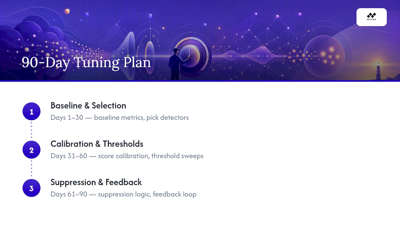
Spend the first 30 days on baseline metrics and detector selection, the next 30 on score calibration and threshold sweeps, and the final 30 building suppression logic and a feedback loop. Skip straight to a monitoring dashboard only after calibration is stable, or you will spend your dashboard budget staring at noise.

Three-stage 90-day anomaly tuning plan

How Netverge Fits Into a Production Tuning Workflow

Netverge is built for the exact architecture this guide recommends, not as a replacement for tuning discipline but as the operational layer that makes it sustainable. Vergepoint hardware gives you the multi-sensor inputs that structural false-positive mitigation depends on, while built-in calibration and AI-driven triage handle the second-stage confirmation step most teams struggle to build in-house.

Netverge

Some AI agents can capture operator feedback directly and feed it back into ongoing tuning, closing the loop described here without extra engineering overhead. The Starter Package runs $299 per month and includes the core monitoring and AI triage stack; additional Vergepoints hardware runs $49 per device per month, and Software Vergepoint access runs $29 per vergepoint per month, both detailed on the pricing guide. If you're running a distributed network and want multi-sensor corroboration without building it from scratch, start a free trial and see how the calibration and suppression layers perform against your own traffic.

Sources

FAQ

Which technique is used for anomaly detection?

There is no single universal technique. Statistical methods like z-score work well for simple seasonal data, Isolation Forest and density methods (LOF, ECOD) suit tabular or multivariate data, and forecaster-plus-residual approaches dominate for time series with strong seasonality.

What are the three types of anomaly detection?

The three broad categories are supervised (trained on labeled normal and anomalous data), semi-supervised (trained mostly on normal data with limited anomaly labels), and unsupervised (no labels, relying on statistical deviation or density). Most production systems, including Netverge's monitoring stack, lean heavily on unsupervised and semi-supervised methods because labeled anomalies are always scarce.

What is the best tool for anomaly detection?

The best tool depends on your data shape and operational constraints rather than any single algorithm. For network and infrastructure monitoring specifically, a platform combining multi-sensor input, calibrated scoring, and second-stage confirmation, the pattern Netverge implements through Vergepoints and AI triage, tends to outperform a standalone detection algorithm running in isolation.

What is the Z-score for anomaly detection?

A z-score measures how many standard deviations a data point sits from the mean of its recent history, and a common starting threshold flags anything beyond 3 standard deviations as anomalous. It works well for simple, roughly normal distributions, but it breaks down on seasonal or skewed data, which is why teams typically layer STL decomposition or a forecaster-plus-residual approach on top of it rather than using a raw z-score alone.